DOI
Authors
License
Publication date
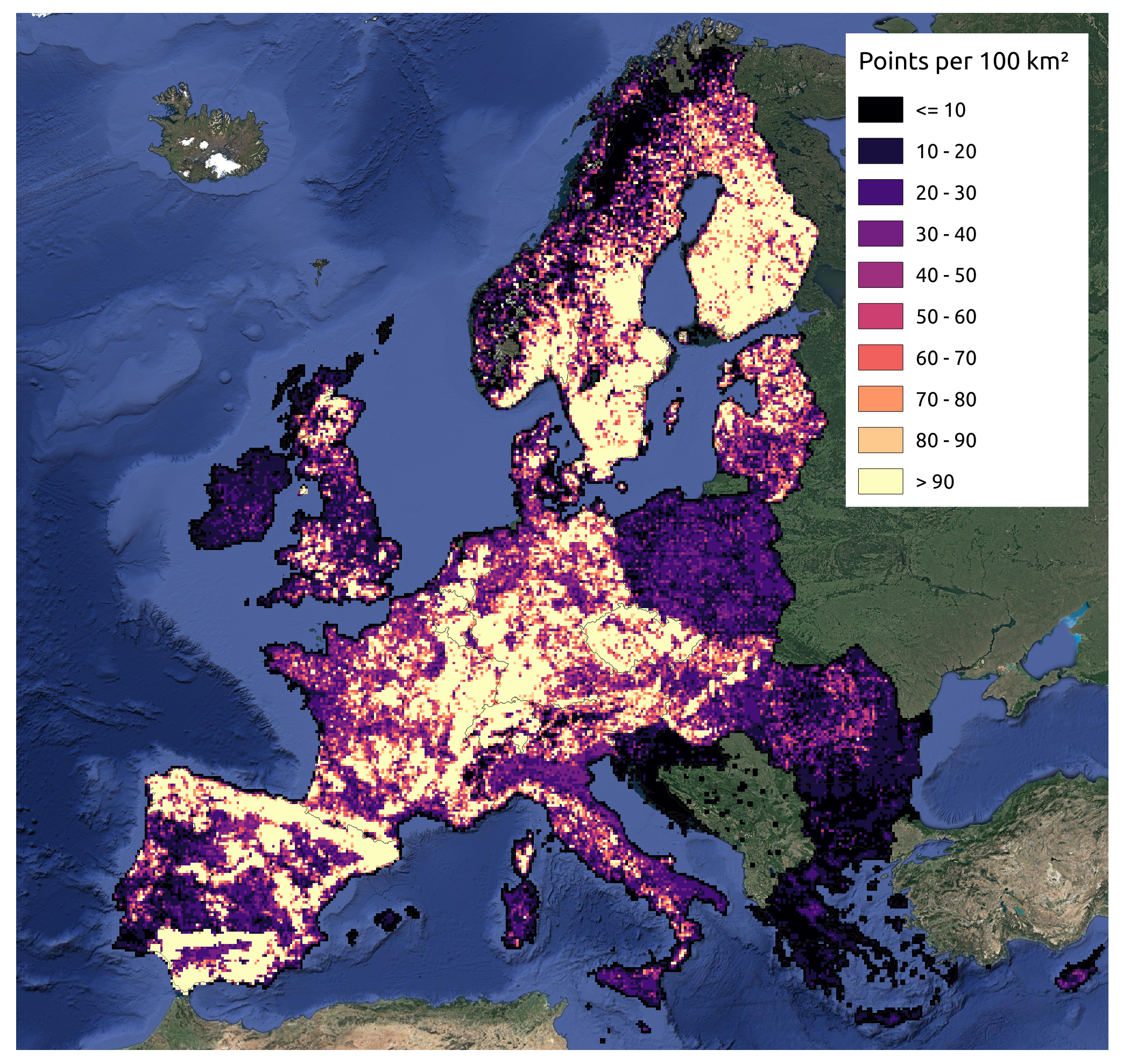
The dataset is a collection of presence and absence points for forest tree species for Europe. Each unique combination of longitude, latitude and year was considered as an independent sample. Presence data was obtained from the harmonized tree species occurrence dataset by Heisig and Hengl (2020) and absence data from the LUCAS (in-situ source) dataset.
The final dataset contains 4,359,999 observations for and a total of 630 columns.
The first 8 columns of the dataset contain metadata information used to uniquely identify the points:
- id: unique point identifier,
- year: year of observation,
- postprocess: quality flag to identify if the temporal reference of an observation comes from the original dataset or is the result of spatiotemporal overlay with forest masks,
- Tile_ID: contains the tile id from the eu_tiling_system (30 km grid),
- easting: longitude coordinates in Coordinate Reference System ETRS89 / LAEA Europe (= EPSG code 3035),
- northing: latitude coordinates in Coordinate Reference System ETRS89 / LAEA Europe (= EPSG code 3035),
- Atlas_class: name of the tree species according to the European Atlas of Forest Tree Species or NULL in case of absence point,
- lc1: contains original LUCAS land cover class or NULL if it's a presence point.
Code on structure and applications of the dataset is available on GitLab
European coverage
EPSG:3035
Bonannella, Carmelo, Hengl, Tomislav, Heisig, Johannes, Leal Parente, Leandro, Wright, Marvin, Herold, Martin, & de Bruin, Sytze. (2022). Presence-Absence Points for Tree Species Distribution Modelling for Europe (0.2) [Data set]. Zenodo. https://doi.org/10.5281/zenodo.5821865
The dataset can be accessed on Zenodo.
					library("curl")
#### Create folder for the project, download files from Zenodo ####

dir.create(paste0(getwd(), "/veg_mapping/"))
setwd(paste0(getwd(), "/veg_mapping/"))

## The whole regression matrix occupies 16 GB on RAM, make sure your workstation can handle it
## Source our custom functions from the script "vegetation_mapping_functions", change the path accordingly

curl_download("https://gitlab.com/geoharmonizer_inea/spatial-layers/-/raw/master/veg_tree.species_anv.pnv.eml/01_dataset_per_species.R?inline=false",
    paste0(getwd(), "/vegetation_mapping_functions.R"))
source("vegetation_mapping_functions.R")

## We use custom functions to read and write RDS files in parallel to speed up processes using pigz
## Functions are customized for Linux systems, you can replace them with the basic, single-core R function
##
## saveRDS.gz -> saveRDS
## readRDS.gz -> readRDS

a.rgr <- curl::curl_download("https://zenodo.org/record/5821865/files/regression_matrix.rds?download=1",
                    tempfile()) %>%
                    readRDS.gz() %>%
                    saveRDS.gz(paste0("01_data/regression_matrix.rds"))