Point data of interest
OpenLandMap.org (previously known under name “LandGIS”) is a system for global soil and vegetation mapping using legacy field observations and state-of-the-art Machine Learning. We use “old legacy data” to produce new added-value information immediately and affordably without new significant investments. We develop procedures to import, clean and reorganize training data, so we can run data mining and spatial predictions to produce finally complete and consistent global maps. With this we also allow for technology and knowledge transfer from data-rich countries to data-poor countries (read more). List of layers currently available via OpenLandMap.org you can track from:
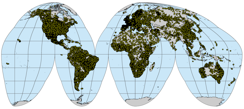
List of training data sets currently used to produce global predictions you can track from:
Why contribute training / point data? If you contribute point data (see example) to some of the workflows used within the OpenLandMap.org project, you contribute to helping make better Open GeoData i.e. better maps of the world i.e. which can be used by everyone (read more about the project backgrounds). Because we automate most of spatial prediction processes, we can continuously update the maps and gradually serve more and more accurate data. The same principle of gradual improvements based on the increasing ground data contributions is followed by, for example, the WorldClim project, OpenStreetMap foundation and/or Global Biodiversity Information Facilities.
In principle, there are three options to contribute point / training data:
- Donate your data to OpenGeoHub foundation,
- Register (DOI) and release your data under some public repository, then share the link to your data with us,
- Provide access to data under a data sharing agreement (to be signed between you and OpenGeoHub),
Here we especially encourage the option (2) i.e. that you register your data and then provide link to us so that we can automate harvesting and use of this data, and attribute your efforts put in maintaining data. For publishing your data we recommended using either: Zenodo.org, HarvardDataVerse, OSF.io and/or Figshare (obtaining a DOI for your data is also highly recommended so that your data can be cited / attributed). Once you register your data, we only need the URL and/or the data set DOI, and we should be able to use it in our workflows. We are also open to signing a data sharing agreement with you, if required, and which is legally binding and will give you more flexibility and protection.
Point data of interest
When uploading and registering your (point or tabular) data you should try to follow some basic principles that will help make your data more usable:
- Remove any unnecessary complexity from your data, especially one that could complicate wider use. For example, use the most simple / most universal format for data or at least non-proprietary format. One simple format for tabular data is for example the Comma Separated Values (CSV).
- Split your data into smaller parts where necessary. Splitting and reorganizing your data can help reduce size (as in any database).
- Compress your data before you upload it to minimize the download time (check your compression ratio using 7z and/or GZIP).
- Attach full description of column names (metadata), which should also include measurement units, detection limit, laboratory / measurement methods and similar (see examples with soil profile observations below).
- Provide spatial (location) and temporal (begin and end observation period) reference and indicate whether the values refer to point samples or bulk samples (mixed material).
- For spatial coordinates best use decimal degrees longitude and latitude in reference to the WGS84 geodetic ellipsoid (EPSG:4326). If you insist on uploading your data in some spatial data format, best use the OGC/GDAL compatible formats such as the GeoPKG.
- Provide most relevant references explaining theory & practice behind observation and measurement of the listed variables.
- Where possible provide measures of accuracy (measurement error / detection limits etc) and confidence (use a scale of 1–10 where 10 is absolutely confident and 1 indicates soft / approximate data).
- Provide (print) snapshots of data and explain how to use and interpret the data (data use tutorials).
Optionally, if you have own infrastructure for serving data, you can serve it through some of the common spatial DB solutions e.g.:
- PostGIS database: You can install point data and then make it available either directly or through Geoserver, so that users can connect to data remotely e.g. by using QGIS.
Harvesting of the data in an online database would be the preferred way of distributing data (assuming that the service is well documented, with plenty of metadata and regularly maintained), but not many organizations can afford this, especially because it requires regular updates and maintenance. If this is the case then cleaning up, exporting and registering the data using some data repository is highly recommended.
Important note: OpenGeoHub provides a publication framework for global environmental data, but is neither the owner nor custodian of Training Data, and therefore is not responsible for the actual content served by Training Data Publishers. OpenGeoHub cannot guarantee the quality or completeness of data, nor does it guarantee uninterrupted data access services. Users employ these data and services at their own risk and in the case of artifacts or inaccuracies will be directed to contact the original Training Data Publishers.
Vegetation / biodiversity data
For global vegetation and biodiversity mapping we primarily use data formats and standards established by the Global Biodiversity Information Facility. This implies the following:
- Data structure for the occurrence data must match the GBIF requirements,
- Taxonomic assignment corresponds to the internationally agreed system,
Ideally, for processing GBIF data you should use the corresponding package (rgbif) as this ensures that the data is up-to-date i.e. that it is directly obtained from GBIF servers (latest snapshot).
OpenLandMap development team is interested in producing maps of actual, historic and potential vegetation at different taxonomic levels e.g.:
- Biomes (highest level; see example),
- Plant communities,
- Individual vegetation species and their traits,
In the case of vegetation species, our requirement is that the GBIF taxonomic ID is set early during the data analysis process. For example, GBIF ID for “Pinus sylvestris – Scots pine” is 5285637. For spatial analysis it is often recommended to remove observations with high location uncertainty, which is often recorded via the columns:
hasGeospatialIssues = FALSE
coordinateUncertaintyInMeters < 2000
which would remove all observations with location error higher than 2 km.
Hengl et al. (2018) shows multiple examples of how to produce distribution maps using vegetation data at various generalization levels. This is an example of biome-class map at 1 km resolution:
pnv_biome.type_biome00k_c_1km_s0..0cm_2000..2017_v0.1.tif
Beyond plant species / community occurrence data, we also help produce global maps of vegetation indices such as the Normalized Difference Vegetation Index (NDVI), Fraction of Absorbed Photosynthetically Active Radiation (FAPAR), Leaf Area Index (LAI) and Dry Matter Productivity (DMP). Here we primarily recommend using standards set by the USGS via their land products derived from their MODIS imagery and Copernicus Global Land Service (CGLS).
Soil data
For global soil mapping we primarily use the National Cooperative Soil Survey (NCSS) Soil Characterization Database as the database model to organize point data and as laboratory methods reference. NCSS SCDB has been chosen because: (a) it is the largest public soil point data resource, and (b) it comes with extensive documentation and examples. In addition, all NCSS data and documentation is available publicly without restrictions and is continuously maintained by USDA / NCSS. To learn how is NCSS SCDB data organized, you can download the Microsoft Access copy of the data, then try adopt your data to its structure and standards. The field survey methods and methods used in the KSSL and other laboratories (e.g., procedures) are documented in detail in “Soil Survey Investigation Report No. 42.” and “Soil Survey Investigation Report No. 45”. To register soil profiles / soil sample datasets please use: https://opengeohub.github.io/SoilSamples/
The NCSS SCDB comprises multiple tables that need to be imported and combined to produce (see import steps) the two standard tables — (1) “sites” table with all information about the site such as coordinates and observation date:
					$ site_key                 : int 12 32 40 48 73 74 85 86 95 99 ...
$ siteiid                  : int 47585 47390 47569 103791 47535 47541 47547 47557 47587 103691 ...
$ usiteid                  : chr "59ND039001" "51ND009009" "59ND003002" "S1953ND103003" ...
$ site_obsdate             : chr "8/20/1959" "9/12/1951" "8/26/1959" "9/16/1953" ...
$ latitude_decimal_degrees : num  47.5 48.8 46.8 47.7 48 ...
$ longitude_decimal_degrees: num  -98.3 -100.7 -98.3 -100 -102 ...
and (2) horizons table with measures / observed soil properties and characteristics per horizon:
					$ layer_key               : int 104 105 106 107 108 109 110 111 112 113 ...
$ labsampnum              : chr "40A00162" "40A00163" "40A00164" "40A00165" ...
$ project_key             : int 1 1 1 1 1 1 1 1 1 1 ...
$ site_key                : int 15 15 15 16 16 16 16 16 16 16 ...
$ pedon_key               : int 15 15 15 16 16 16 16 16 16 16 ...
$ layer_sequence          : int 5 6 7 1 2 3 4 5 6 7 ...
$ layer_type              : chr "horizon" "horizon" "horizon" "horizon" ...
$ hzn_top                 : num 66 84 117 0 13 18 41 61 91 122 ...
$ hzn_bot                 : num 84 117 152 13 18 41 61 91 122 183 ...
$ hzn_desgn               : chr "Bk2" "C1" "C2" "Ap" ...
$ cec7_cly                : num 1.04 0.84 1.06 1.01 0.79 ...
$ w15cly                  : num 0.74 0.68 0.88 NA NA ...
...
The two tables can be bind via the “site_key” column. Detailed description of the columns in the NCSS SCDB can be found in the table NCSS_Data_Dictionary_Layer.csv (site variables) and NCSS_Data_Dictionary_Data_Tier.csv (chemical and physical properties); the analysis procedures are further listed in NCSS_Analysis_Procedure.csv. The column name “ph_h2o” (pH, 1:1 Soil-Water Suspension), for example, was used to produce global map of soil acidity at 250 m:
sol_ph.h2o_usda.4c1a2a_m_250m_b*..*cm_1950..2017_v0.2.tif
Code “usda.4c1a2a” indicates that these the reference laboratory method is “4C1a2a” which is explained in detail in “Soil Survey Investigation Report No. 42.” and “b10..10cm” indicates that the predictions refer to 10 cm below ground. If you are in possession of similar soil data (field surveys and laboratory analyses) we can add your points to existing mapping framework and then use them to produce better soil maps of the world.
If you do not have capacity or resources to convert, standardize and harmonize soil / field point data yourself, you can also forward your data in the original format. Provided that we receive enough metadata, and provided that your data is significant (≫100 rows), we will create and publish import code that explains necessary renaming of columns and conversion of values, and then use your data to help improve overall accuracy of the maps. All processing steps and improvements you will be able to follow via the https://gitlab.com/openlandmap / version control system (for examples renaming on the columns to match the NCSS names), so that you can also comment and participate in the processing steps. An example of import and harmonization steps you can find here.